Activation Functions

An activation function is the small mathematical curve applied at each neuron. After a neuron adds up its weighted inputs, the activation function reshapes that sum into the neuron's output. This non-linear reshaping is what gives a neural network its ability to model curves and interactions rather than just straight-line relationships — without it, stacking layers would be no more powerful than a single linear formula.

You choose the activation for each layer of an MLP with the SetNetworkWithActivationLayer1…4 functions described on the Network Architectures page. Each function takes the hidden-layer activations as the second item of each (neurons, activation) pair, and the output-layer activation as the final argument. If you use the plain SetNetworkLayer… functions instead, every layer defaults to Sigmoid.

The activation codes

The activation is selected by an integer code. The full set is below.

Code	Activation — when to use
0	Sigmoid (logistic) — saturating, outputs 0..1. Good as an output activation for probabilities / classification (up vs down).
1	Tanh — saturating, outputs −1..1, zero-centred. A solid, reliable general-purpose hidden activation.
2	Symmetric Elliot — a cheaper, tanh-like sigmoid in the −1..1 range.
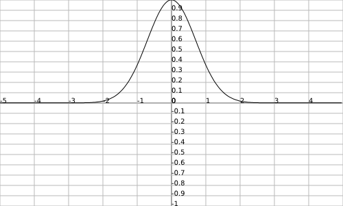
3	Symmetric Gaussian — a bell-shaped response in a symmetric range; specialised, for localised patterns.
4	Elliot — a cheaper, faster approximation of the sigmoid in the 0..1 range.
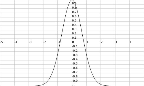
5	Gaussian — bell-shaped response; specialised.
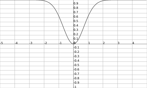
6	Inverse Gaussian — an inverted bell; specialised.
7	ReLU — non-saturating; passes positives through, zeroes negatives. A strong modern choice for hidden layers; pair with He weight initialisation.
8	LeakyReLU — like ReLU but lets a small slope through on the negative side, avoiding "dead" neurons. A safe alternative to ReLU for hidden layers.
9	Linear (identity) — passes the value straight through with no limit. The recommended output activation for regression, where the prediction can be any value.

Saturating vs. non-saturating

The activations fall into two broad groups, and the distinction matters in practice.

Saturating activations (sigmoid, tanh, the Elliot and Gaussian variants) squash their output into a fixed range and flatten out at the extremes. They are smooth and well-behaved and have been the classic choice for hidden layers. Their weakness is that very large inputs push them into their flat regions, where learning slows down.

Non-saturating activations (ReLU and LeakyReLU) do not flatten on the positive side, which keeps learning brisk in deeper networks. ReLU can occasionally leave neurons permanently stuck at zero ("dead units"); LeakyReLU avoids this by allowing a small negative slope. These pair naturally with He weight initialisation (see Accuracy & Avoiding Overfitting).

Tip

For a regression network that predicts an unbounded value (such as a future return), use a saturating or ReLU activation on the hidden layers and a Linear output (code 9). If the output stays a saturating function such as sigmoid, the prediction is trapped in 0..1 and can never reach the values you want. For classification (a 0..1 probability), use a Sigmoid output (code 0) together with the Tanh loss — see Accuracy & Avoiding Overfitting.

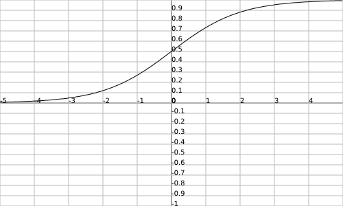
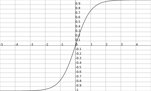
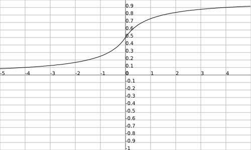
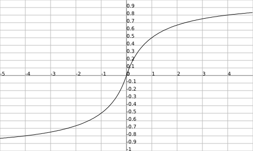
Shapes of the saturating activations

The images below show the shape of each saturating activation — the curve that maps the neuron's summed input (horizontal axis) to its output (vertical axis).

The logistic (sigmoid) activation curve, an S-shape rising from 0 to 1. — Sigmoid (logistic) — code 0. Outputs 0..1.

The tanh activation curve, an S-shape rising from -1 to 1. — Tanh — code 1. Outputs −1..1, zero-centred.

The Elliot activation curve, a sigmoid-like S-shape in the 0 to 1 range. — Elliot — code 4. A cheaper sigmoid-like curve, 0..1.

The symmetric Elliot activation curve, a tanh-like S-shape in the -1 to 1 range. — Symmetric Elliot — code 2. A cheaper tanh-like curve, −1..1.

The Gaussian activation curve, a bell shape. — Gaussian — code 5. A bell-shaped response.

The symmetric Gaussian activation curve, a symmetric bell shape. — Symmetric Gaussian — code 3.

The inverse Gaussian activation curve, an inverted bell shape. — Inverse Gaussian — code 6.

Note

Activations are an MLP feature. The recurrent LSTM and GRU models use fixed internal gate activations and a linear output, so the codes above do not apply to them.