Introduction to Neural Networks

The WiseTrader Toolbox lets you build, train and run neural networks directly from AFL. A neural network is a flexible pattern-matching tool: you show it examples of some inputs (indicators, lagged prices, returns, volume, anything you can compute in AFL) alongside the target you want it to predict, and it learns the relationship between them. Once trained, you can apply that network to new bars to produce a prediction.

In plain trading terms, a neural network is a non-linear way to combine several indicators into a single output. Where a moving-average crossover or a simple weighted score uses a fixed formula you chose yourself, a neural network discovers the weighting from your historical data — including non-linear interactions that would be hard to write by hand.

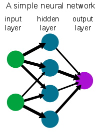
A network is organised in layers: an input layer (one neuron per input you supply), one or more hidden layers that do the actual pattern-finding, and an output layer (the prediction). The more hidden layers and neurons you add, the more complicated a relationship the network can represent — but also the more easily it can go wrong, as explained below.

The train → predict workflow

Working with a network always has two phases:

1. Training. The network studies your historical data and adjusts its internal weights until its predictions match the target as closely as it can. You do this once and the trained network is saved to a file.
2. Prediction. You load the saved network and apply it to new bars to generate predictions, with no further learning.

You control everything by calling Set... configuration functions in your AFL before you train. These choose the network size, the training algorithm, how the data is scaled, and the settings that keep predictions honest. A full list is on the Settings Reference page, and the training and prediction functions themselves are documented under Neural Network Functions.

The three-section AFL formula pattern

Almost every neural-network formula you write follows the same three-part shape. Keeping to this pattern makes formulas easy to read and avoids settings leaking from one formula into the next.

1. Settings. Call the Set... functions that configure the network (size, activations, training algorithm, scaling, anti-overfitting options).
2. Inputs, output and train/run. Build your input and target arrays and pass them to a training or prediction function.
3. Cleanup. Call RestoreDefaults() at the end so the next formula starts from a clean slate.

// 1. Settings
SetLearningAlgorithm( 4 );                 // iRPROP+ (robust default)
SetNetworkWithActivationLayer1( 8, 1, 9 ); // 8 tanh hidden neurons, linear output
SetPercentTestingData( 25 );               // hold back 25% to detect overfitting
SetEarlyStoppingPatience( 30 );
SetMaximumEpochs( 300 );

// 2. Inputs, output and train
input1 = PercentDifference( Close, 1 );    // rate of change, not raw price
input2 = RSI( 14 ) / 100;
target = Ref( PercentDifference( Close, 1 ), 1 );  // tomorrow's change
TrainNeuralNetwork3( input1, input2, target, "MyNetwork" );

// 3. Cleanup
RestoreDefaults();

Standard networks vs. Walk-Forward networks

The toolbox offers two ways of working with networks, and it is worth knowing the difference before you start.

Standard networks use the TrainNeuralNetwork… / RunNeuralNetwork… family (and their multi-input equivalents). You train one network on a block of history, save it to a named file, and later run it. Training and prediction are two separate steps you control. This is the most flexible approach and supports every feature, including the recurrent LSTM and GRU models.

Walk-Forward networks use the NeuralNetworkIndicator… family. These do everything in a single call: as the indicator walks along the chart, it repeatedly trains a fresh short-lived network on the bars immediately before each bar and predicts a chosen number of bars ahead. Because each prediction only ever sees past data, the result is genuinely out-of-sample at every bar — which makes it a realistic picture of how the model would have behaved in real time. The trade-off is that it is heavier to compute and is limited to the feed-forward MLP model.

The single most important idea: overfitting

If you remember only one thing from this manual, make it this. The biggest risk with any neural network is overfitting: the network memorises the quirks and random noise of the training data instead of learning the real, repeatable pattern. An overfit network looks fantastic on the data it trained on and performs poorly on new bars — which is the only thing that matters for trading.

Neural networks are powerful precisely because they can model very complex relationships, and that same power is what lets them memorise noise. A network with too many neurons, trained for too long, on too little data, will almost always overfit. The good news is that this is controllable. The toolbox publishes two numbers after training — NeuralNetworkMSE (error on the training data) and TestingDataNeuralNetworkMSE (error on held-out data) — so you can actually see overfitting happening, and it gives you a set of tools to fight it.

Garbage in, garbage out

A neural network is not magic. It can only find a relationship between your inputs and your target if one genuinely exists. Choosing good inputs and a sensible, predictable target is the most important creative work you do — the network simply finds the best combination of whatever you give it.

One practical consequence stands out for traders. Internally the network works best with data in a small, stable range, and it scales your data automatically. Raw price is a poor input because it drifts over time — a stock that traded at $0.10 years ago and $30 today has no stable range, so a network trained on it predicts poorly. Feed the network a rate of change (for example the percent change of the Close, via PercentDifference) instead of the raw price. A rate of change stays in a roughly constant range over the whole history and gives far more reliable predictions. This and the related scaling settings are covered on the Input & Output Scaling page.

A more reliable use: filtering signals

Predicting price or the next return — what most people try first — is genuinely hard, and the tutorials are honest about how thin the signal usually is. There is a more accessible use that tends to work much better: keep a trading system you already have and use a network to filter its signals, keeping the entries that look like winners and dropping the likely losers. You are handing the network an easier, better-posed question — "is this signal likely to win?" — instead of asking it to forecast the market from scratch.