Accuracy Tab

Think of the Accuracy tab as one tab with one job: stop the network memorising the past. These are the regularization controls — the settings that fight overfitting and keep training stable. With financial data, where the signal is weak and noisy, they matter more than raw network size. A smaller, well-regularized network beats a big one that has memorised history almost every time.

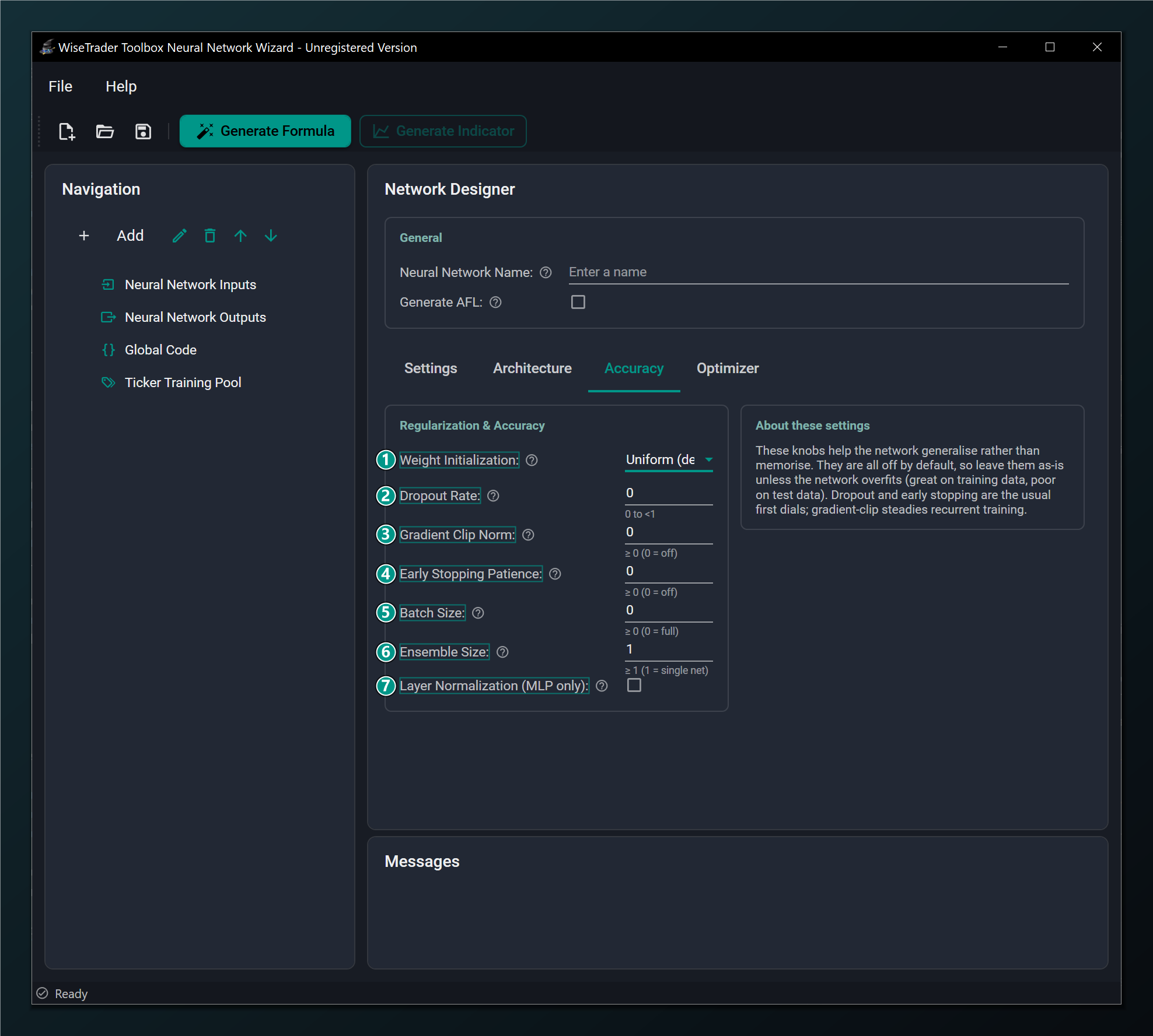
1. Weight Initialization — how starting weights are drawn. Uniform (original), Xavier (tanh/sigmoid) or He (ReLU).
2. Dropout Rate — randomly drops this fraction of units during training to curb overfitting. 0 = off.
3. Gradient Clip Norm — caps the size of weight updates to keep training stable (helps recurrent nets). 0 = off.
4. Early Stopping Patience — stop early if the test score has not improved for this many epochs. 0 = disabled.
5. Batch Size — rows per gradient step for the stochastic optimizers. 0 = full batch.
6. Ensemble Size — 1 = one network; k>1 trains k seed-varied networks and averages their predictions (more robust, ~k× slower). Works with any model type; disables AFL export when above 1. Default 1.
7. Layer Normalization (MLP only) — adds LayerNorm to every hidden layer of an MLP to stabilise/speed up training of deeper nets. Shown for MLPs only; disables AFL export when on. Default off.

Weight Initialization: where training starts

Training begins from random weights, and where it starts affects how smoothly it gets going. The trick is to scale those random starting numbers to the size of each layer so the signal neither fades to nothing nor blows up as it flows through. The right scheme depends on the activation you chose:

• Uniform — the original, simple scheme. A safe baseline.
• Xavier — tuned for TanH / sigmoid layers.
• He — tuned for ReLU / Leaky ReLU layers.

Default is Uniform. It won't break anything, but matching the scheme to your activation makes training converge faster and more reliably — pick Xavier for tanh/sigmoid networks, He for ReLU networks.

Dropout Rate: forcing the network to generalise

Dropout is a clever anti-memorisation trick. During each training step it randomly switches off a fraction of the neurons, so the network can never lean too hard on any single one and has to spread what it learns across many. It's like quizzing a study group with a few members randomly absent each round — everyone has to actually understand the material rather than rely on one know-it-all. The result is a network that leans on robust, repeatable patterns instead of memorised quirks.

The value is the fraction dropped: 0 = off (the default), and you can go up to (but not including) 1. On larger networks, 0.1–0.5 is the useful band; small networks often need none. Turn it on if the test error is much worse than the training error — the signature of overfitting.

Gradient Clip Norm: keeping training stable

Occasionally a single training step produces a wildly large update that throws the network off course — an "exploding" update. Gradient clipping puts a ceiling on how big any one update can be, so training stays on the rails. 0 = off (default); any positive number sets the cap. You rarely need it for plain MLPs, but it is genuinely useful for recurrent (LSTM/GRU) models, which are prone to these blow-ups. If a recurrent net's error suddenly spikes to nonsense, switch this on (try a value around 1–5).

Early Stopping Patience: quit while you're ahead

This is the most direct cure for overfitting on the tab, and a free speed-up. As training runs, the Wizard watches the error on your held-out test set. That error falls while the network is genuinely learning, then starts rising once it begins memorising noise — the moment you want to stop. Early stopping ends training automatically if the test score hasn't improved for this many epochs in a row.

0 = disabled (default). A value like 20–50 is a sound choice: it lets you set a generous epoch cap and trust early stopping to halt at the sweet spot, saving time and guarding against overtraining.

Batch Size: how many bars per learning step

The stochastic (Adam-family) optimizers can update the weights after looking at a small batch of rows rather than the whole dataset at once. 0 = full batch (default): every step uses all the rows, which is steady but slower. A small positive value — say 32 or 64 — means the network learns from many little samples instead, which speeds training up and adds a dash of helpful randomness that can itself reduce overfitting. Only the stochastic optimizers honour this; under classic BackPropagation it has no effect.

Ensemble Size: many nets, one steadier answer

Ensemble Size trades training time for robustness, and it works with any model type. Leave it at 1 (the default) for a single network. Set it to k>1 and the Wizard trains k networks that differ only in their random seed, then averages their predictions. Because each member starts from a different place and makes slightly different mistakes, the average cancels much of that idiosyncratic noise — the same reason a panel of forecasters beats any one of them. The cost is roughly k× the training time. At run time the formula auto-discovers the saved members and blends them for you.

A modest ensemble (3–5) is a cheap, reliable way to firm up a prediction that swings too much from one training run to the next. Above 1, network-to-AFL export is switched off (an ensemble can't be folded into a single formula).

Layer Normalization: steadier training for MLPs

Layer Normalization is a default-off toggle that adds a LayerNorm step to every hidden layer of an MLP (the output layer is never normalised). It re-centres and re-scales each layer's activations as they flow through, which keeps the signal in a healthy range and makes training of deeper MLPs steadier and often faster. It is most worth trying when a multi-layer network trains sluggishly or unevenly; a small one- or two-layer network rarely needs it.

It is shown for MLPs only — the sequence models handle their own normalisation internally, so the toggle is hidden for them. Turning it on disables network-to-AFL export.