Architecture Tab
The Architecture tab is where you choose the model type and lay out its hidden layers. The default — a Feed-Forward (MLP) network — is robust and a good starting point; the other four model types (LSTM, GRU, TCN and Transformer) are sequence models that read a window of bars in order and suit sequence-aware predictions. The tab shows exactly one model-parameter editor at a time — the MLP layer editor, the recurrent fields, the TCN fields or the Transformer fields — depending on the model type you pick.
Layers, neurons and activations — in plain English
Three words appear all over this tab. Here's what they actually mean, with no maths.
- A neuron is a tiny calculator. It takes the numbers coming into it, weighs each one, adds them up, and passes the total through an activation function to produce a single output. One neuron on its own is simple; the power comes from wiring many together.
- A layer is a row of neurons that all see the same inputs. Your network has an input layer (one slot per input you feed it), one or more hidden layers that do the real pattern-finding, and an output layer that produces the prediction.
- An activation function is the bend in each neuron. Without it, no matter how many neurons you stack, the whole network could only draw straight lines — the same as a plain weighted average. The activation is what lets the network learn curved, non-linear relationships, which is the entire reason to use one over a hand-written indicator formula.
So configuring the architecture is really just deciding how much brain to give the network: how many neurons, in how many layers, with what kind of bend. More brain can learn more complex patterns — and overfit more easily, the cardinal sin for traders.
Feed-Forward (MLP)
A Feed-Forward network — the classic Multi-Layer Perceptron — passes data straight through, input layer to hidden layers to output, with no memory of previous bars. It is fast, robust, supports every training algorithm and feature, and is the right choice for almost everything. Start here.
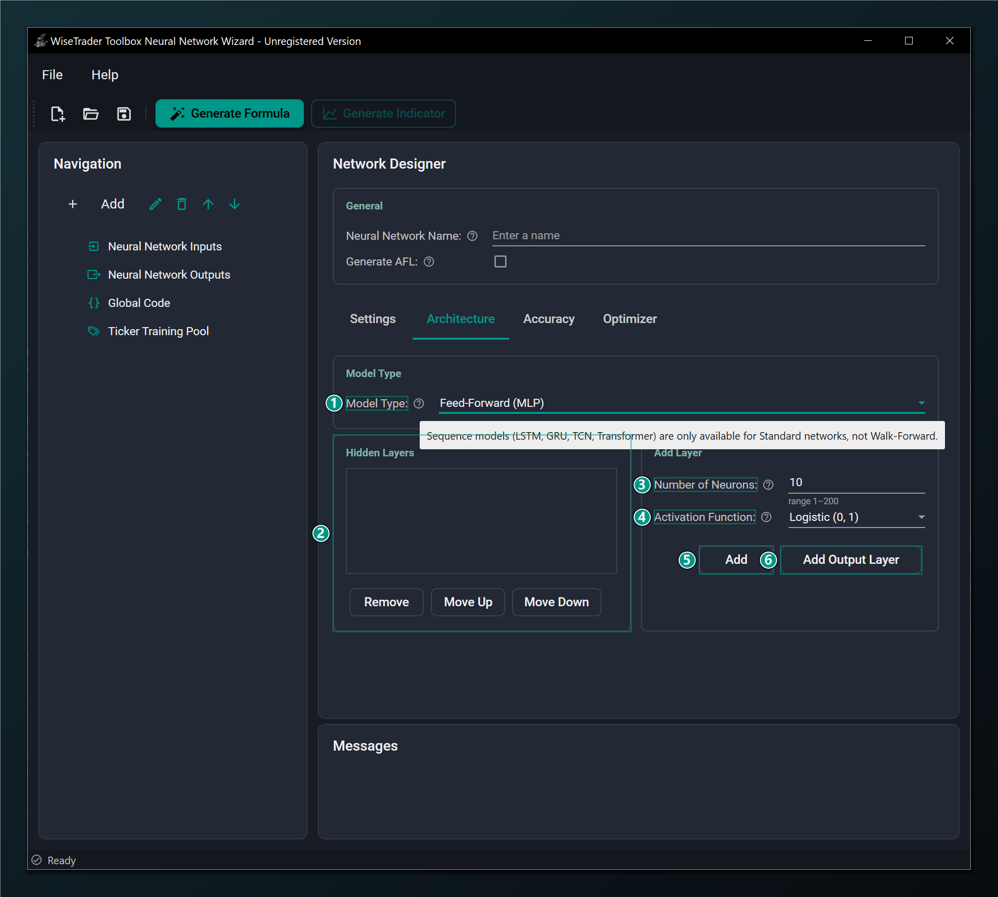
- Model Type — Feed-Forward (MLP) is the robust default; LSTM, GRU, TCN and Transformer are sequence models (Standard-only).
- Hidden Layers — the list of hidden layers in order, input to output. Select one to remove or reorder it.
- Number of Neurons — neurons in this hidden layer. More = more capacity but slower and easier to overfit. Default 10.
- Activation Function — shapes a layer's output; match it to your output scaling.
- Add — adds one hidden layer with the neurons/activation above (up to 4 hidden layers).
- Add Output Layer — adds the final output layer (one only); its activation sets the output range.
Number of Neurons and Hidden Layers
Together these set the network's capacity — how complicated a relationship it can represent. The temptation is to add lots, on the theory that bigger is smarter. With noisy financial data the opposite is usually true: a big network has more than enough freedom to memorise the past and predict the future poorly.
Number of Neurons sizes one hidden layer (default 10, range 1–200). You can stack up to 4 hidden layers, added in order from input to output. A practical recipe for the markets: start with a single hidden layer of a handful of neurons (say 4–10). Only add a second layer or more neurons if a smaller network plainly underfits — that is, if it can't even fit the training data well.
Start small. One or two hidden layers of a handful of neurons each is usually enough for financial data; piling on neurons and layers mostly buys you overfitting. Add capacity only when a smaller network plainly underfits.
Activation Function
The activation sets the shape — and the output range — of a layer. The choice matters in two places. For hidden layers, modern unbounded activations like ReLU or Leaky ReLU train quickly and are a fine default; the classic TanH also works well. For the output layer, the activation decides what range the prediction can land in, and that has to line up with how you scaled the target:
| Activation | Output range | Use for |
|---|---|---|
| Logistic / Elliot / Gaussian | (0, 1) | Hidden layers, or outputs scaled to (0, 1) |
| TanH / Symmetric | (−1, 1) | Hidden layers, or outputs scaled to (−1, 1) |
| ReLU / Leaky ReLU / Linear | unbounded | Hidden layers, and regression outputs that can be any value |
The output activation and your Output Data Scaling must agree. A bounded activation can only ever emit numbers inside its range, so a TanH output with a target scaled to (0, 1) — or vice versa — can never reach the answer and training fails quietly. For plain price/return regression, a Linear output is the safe pick. See Output Data Scaling on the Settings tab.
Choosing the model type
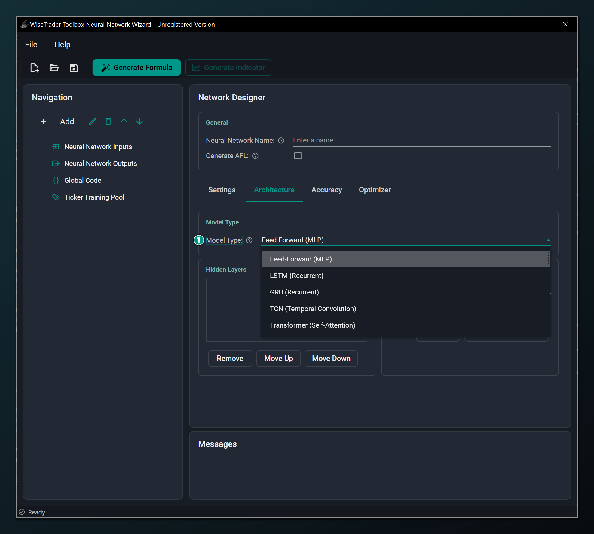
- Model Type list — Feed-Forward (MLP), LSTM and GRU (recurrent), TCN (temporal convolution) and Transformer (self-attention). The four non-MLP types are sequence models that read a window of bars in order; they are Standard-only (no Walk-Forward, no AFL export).
Feed-Forward vs. the sequence models
The difference is memory. A Feed-Forward network treats each bar independently — whatever history you want it to see, you have to hand it yourself via lagged inputs. A sequence model reads a sequence of consecutive bars in order, so it can pick up on the shape of recent price action on its own. LSTM, GRU, TCN and Transformer are four different ways of doing that.
- Feed-Forward (MLP) — no memory, fast and robust, every feature available. The best choice for almost everything. Reach for it first.
- LSTM — Long Short-Term Memory, the more powerful recurrent model. Its gated memory cell can hold information across many bars, useful when the order and rhythm of recent bars carries the signal. Trains with the Adam-family optimizers.
- GRU — Gated Recurrent Unit, a streamlined cousin of LSTM with fewer gates. Trains a little faster and often performs comparably, especially on shorter windows.
- TCN — Temporal Convolution, a causal, dilated 1-D convolution that reads the whole window in parallel rather than stepping through it. Its receptive field grows quickly with depth, so it can see a long history cheaply.
- Transformer — a causal multi-head self-attention encoder, the most expressive sequence model: it weighs every bar in the window against the others. It benefits from more data.
When would a trader pick a sequence model? When you suspect the predictive information is in the sequence of recent bars — the path price took, not just a snapshot of indicators today. For most indicator-based systems a Feed-Forward network with a few lagged inputs does the job with far less fuss. All four sequence models are Standard networks only: no Walk-Forward, and no network-to-AFL export; they train with the Adam-family / RMSProp optimizers rather than the RPROP family.
LSTM & GRU (recurrent networks)
Selecting LSTM or GRU turns the network into a recurrent one that reads a window of consecutive bars in order through a gated memory cell. The layer editor is replaced by a few recurrent-specific fields.
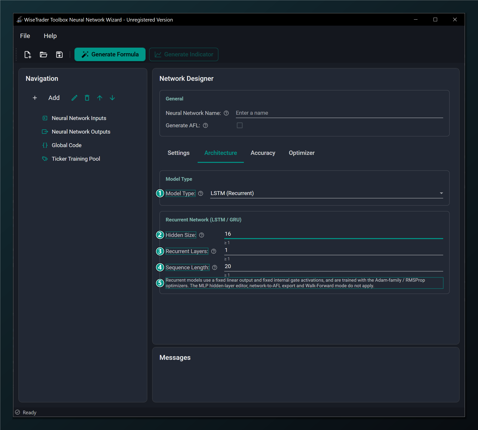
- Model Type = LSTM (Recurrent) — reads a window of consecutive bars in order with a gated memory cell. Standard networks only; selecting it auto-switches the optimizer to AdamW.
- Hidden Size — units in the recurrent cell (the size of its memory). Larger models more complex dynamics but overfits more easily. Default 16.
- Recurrent Layers — number of stacked recurrent layers; a value above 1 builds a genuinely deeper (stacked) network. 1 is the usual choice. Default 1.
- Sequence Length — how many consecutive bars the network reads as one sequence before predicting. Default 20.
- Recurrent restrictions — fixed linear output and gate activations, Adam-family optimizers only; the MLP layer editor, network-to-AFL export and Walk-Forward mode do not apply.
Hidden Size, Recurrent Layers and Sequence Length
These three are the recurrent equivalent of "how much brain and how much history".
- Hidden Size is the size of the memory — how much the cell can remember at once. Bigger captures richer dynamics but overfits more easily. Default 16 (1 or greater); 16–64 is a sensible band to explore.
- Recurrent Layers stacks one cell on top of another — a value above 1 builds a genuinely deeper, stacked RNN. 1 is almost always right for market data; add a second only if a single layer clearly underfits. Default 1.
- Sequence Length is how many consecutive bars the network reads before it predicts — its window of history. This is the recurrent counterpart of an MLP's lag range. Default 20 (1 or greater): roughly a month of daily bars. Match it to the horizon over which you think recent history matters.
Recurrent models are Standard networks only. They cannot be used in Walk-Forward mode, and selecting one auto-switches the learning algorithm to AdamW. Network-to-AFL export is also unavailable for recurrent networks.
TCN (temporal convolution)
Selecting TCN turns the network into a causal, dilated 1-D convolution that reads a window of bars in parallel. Like the recurrent models it replaces the MLP layer editor with its own fields, and it shows a live, read-only receptive field hint so you can see how far back the network sees as you tune it.
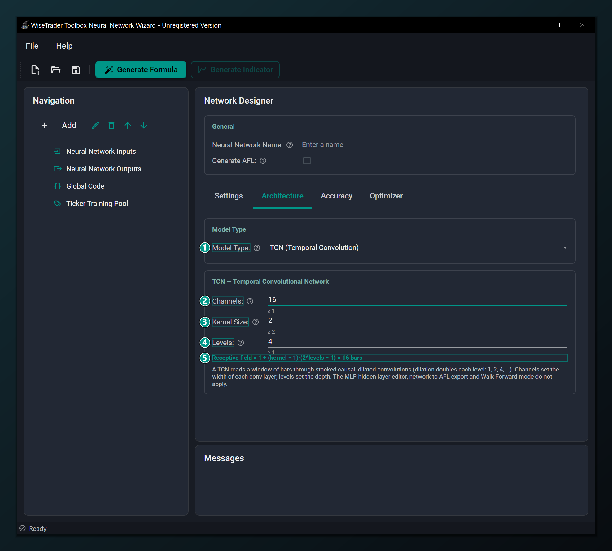
- Model Type = TCN (Temporal Convolution) — a causal, dilated 1-D convolution that reads a window of bars in parallel. Standard networks only; trains with the Adam-family optimizers; the MLP layer editor, AFL export and Walk-Forward mode do not apply.
- Channels — width of each convolution layer (its feature channels). More = more capacity but slower. Default 16; must be 1 or greater.
- Kernel Size — convolution kernel width. With Levels it sets how far back the network sees (dilation doubles each level: 1, 2, 4, ...). Default 2; must be 2 or greater.
- Levels — number of stacked dilated convolution levels (the depth). Each added level roughly doubles the receptive field. Default 4; must be 1 or greater.
- Receptive field — the read-only window length the TCN reads, computed as 1 + (kernel − 1)(2^levels − 1) bars; it updates live as you change Kernel Size or Levels.
Channels, Kernel Size and Levels
Channels is the TCN's "how much brain" — the width of each layer
(default 16, 1 or greater). Kernel Size and
Levels together set its "how much history": because each level doubles
the dilation (1, 2, 4, 8, ...), the network's reach grows fast with depth. The
Receptive field hint reads out the exact window in bars —
1 + (kernel − 1)(2^levels − 1) — so you can match it to the
horizon you care about. With the defaults (kernel 2, levels 4) that is 16 bars; raise
Levels to reach further back cheaply.
Transformer (self-attention)
Selecting Transformer turns the network into a causal multi-head self-attention encoder — the most expressive sequence model. It has its own fields and a live, read-only head size hint that flips to a warning when the model dimension is not divisible by the head count.
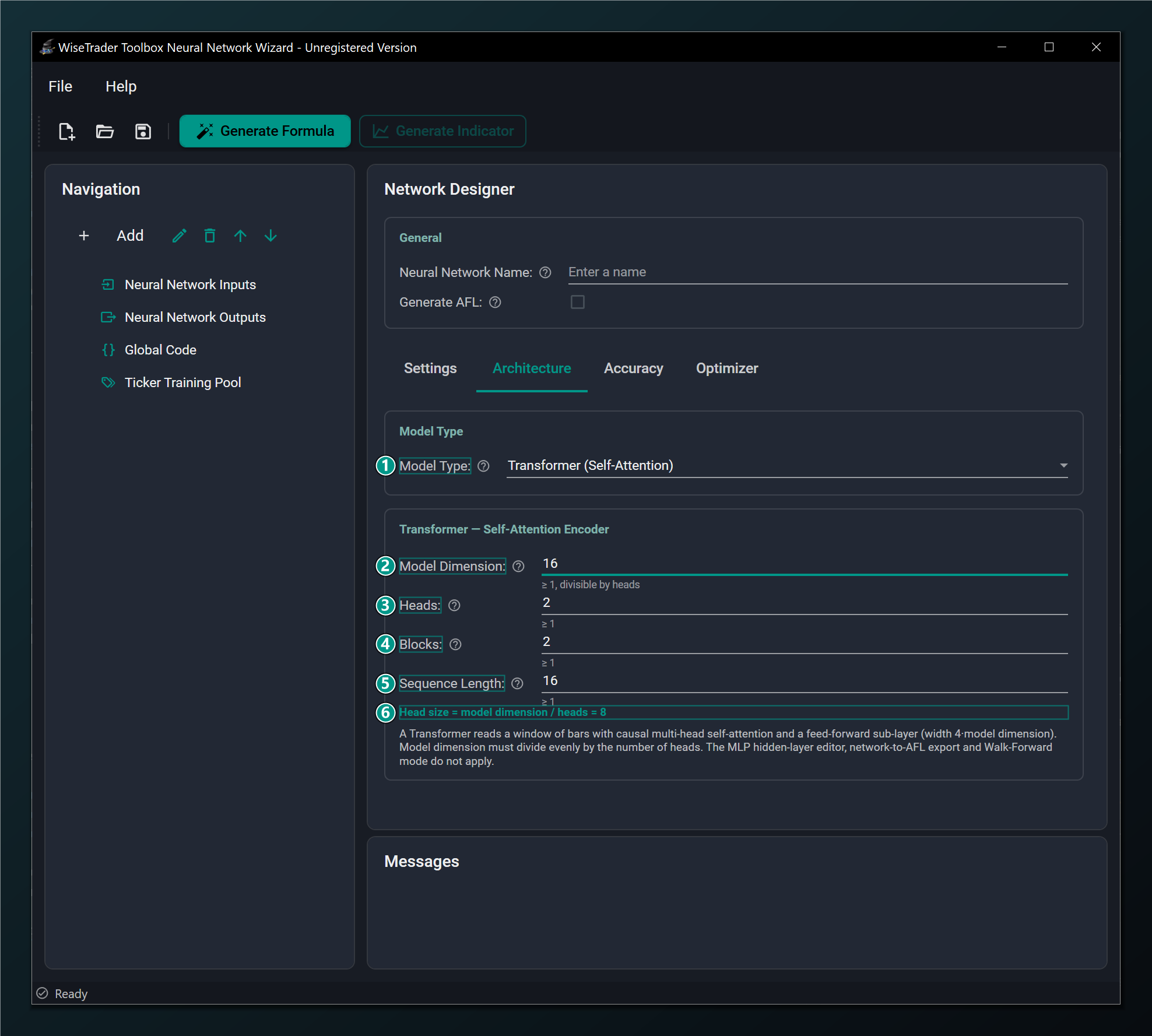
- Model Type = Transformer (Self-Attention) — a causal multi-head self-attention encoder. The most expressive sequence model; Standard networks only; the MLP layer editor, AFL export and Walk-Forward mode do not apply.
- Model Dimension — width of the attention/embedding vectors. Must divide evenly by the number of heads. Default 16; must be 1 or greater.
- Heads — number of attention heads the model dimension is split across; each attends to a different sub-space. Default 2; must be 1 or greater.
- Blocks — number of stacked encoder blocks (the depth). More = more expressive but slower and hungrier for data. Default 2; must be 1 or greater.
- Sequence Length — how many consecutive bars the encoder reads as one sequence before predicting. Default 16; must be 1 or greater.
- Head size — the read-only model-dimension / heads value; it flips to a warning when the model dimension is not divisible by the head count (which the validator rejects).
Model Dimension, Heads, Blocks and Sequence Length
Model Dimension is the width of the attention vectors (default 16) and Blocks is the depth (default 2) — together the Transformer's capacity. Heads (default 2) splits that width into independent attention sub-spaces, so the model dimension must divide evenly by the head count; the Head size read-out shows the result and warns you when it doesn't divide. Sequence Length (default 16) is the window of bars the encoder reads at once — the Transformer counterpart of the recurrent models' sequence length. Being the most expressive model, it benefits from more data; start small and lean on the Accuracy tab.
For a Transformer, the Model Dimension must be divisible by the number of Heads. If it isn't, the Head size hint turns into a warning and the network won't validate — pick a head count that divides the model dimension evenly (for example 16 / 2 = 8).
Optimizer fields under a sequence model
Because the sequence models (LSTM, GRU, TCN and Transformer) train with the Adam-family / RMSProp optimizers, the Optimizer tab shows their hyperparameters directly. The learning-rate schedule and Batch Size apply to every model type, sequence models included.
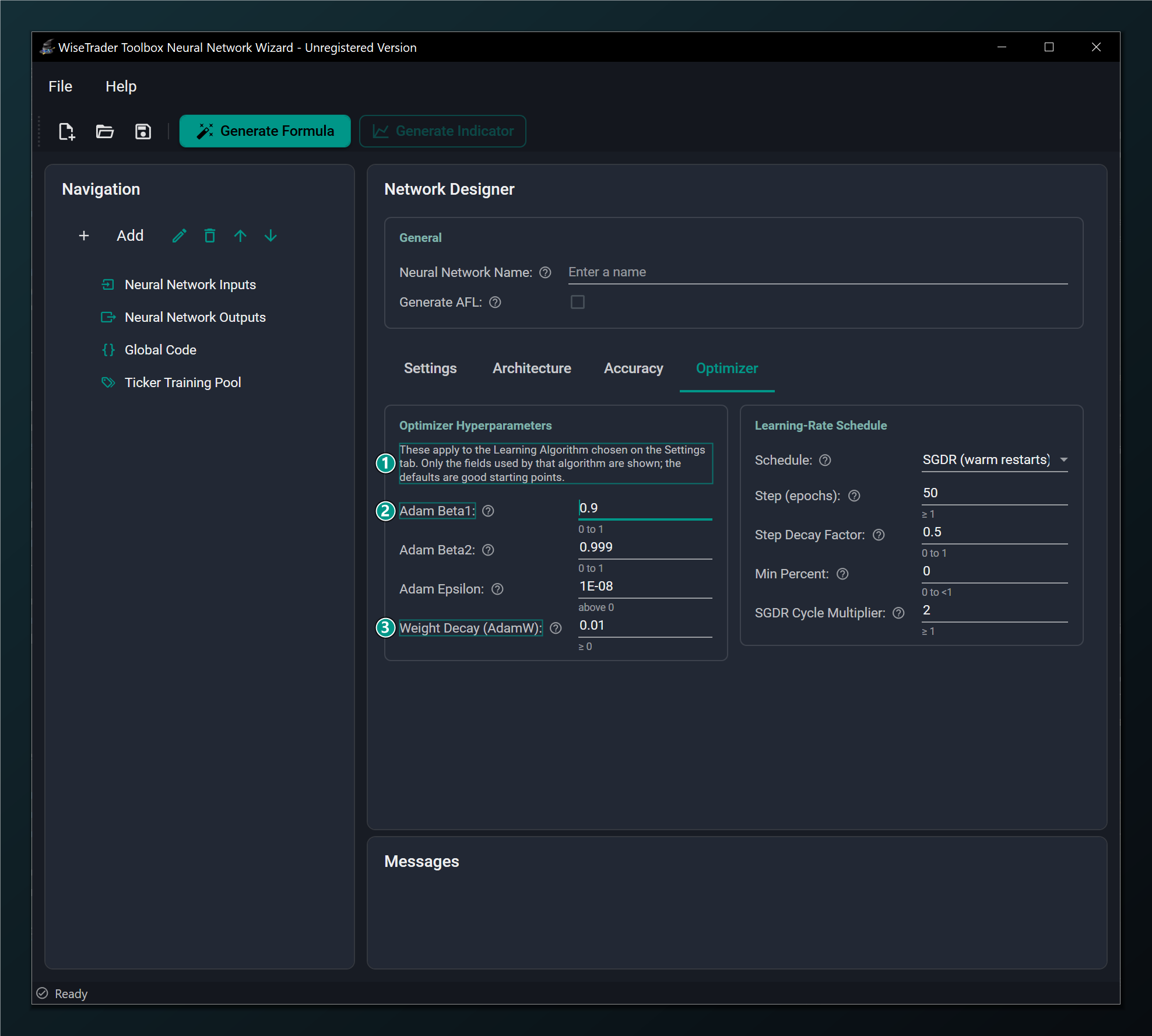
- Adam-family hyperparameters — sequence models train with the Adam-family / RMSProp optimizers, so their hyperparameters are shown here.
- Adam Beta1 — momentum decay for the running gradient average. Default 0.9.
- Weight Decay (AdamW) — the AdamW regularization strength; the Learning-Rate Schedule box on the right remains available for sequence models too.
Sequence models also pair naturally with Gradient Clip Norm on the Accuracy tab, which keeps their training stable, and they need Randomly Shuffle Data left off so the bar order they depend on is preserved.