Settings Tab

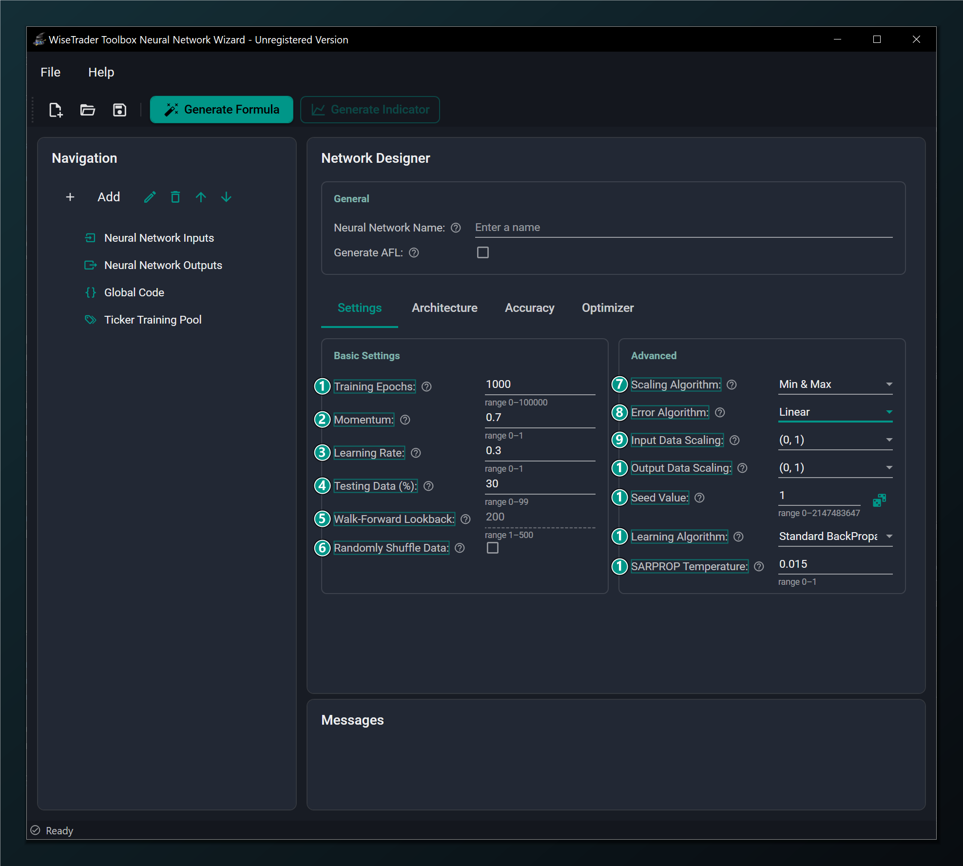
The Settings tab holds the core training controls. It is split into two groups: Basic Settings on the left (how long and how fast the network trains, the test split) and Advanced on the right (how data is scaled, and the error and learning algorithms). New to the vocabulary here? Skim Neural Networks for Traders first — it explains training, prediction and overfitting in plain English.

Basic Settings

The left-hand group (callouts 1–6) controls how long and how fast the network trains and how it is tested.

1. Training Epochs — max passes over the data while training. Higher learns more but is slower and can overfit. Default 1000.
2. Momentum — smooths weight updates using the previous step to speed up and steady training. Default 0.7 (range 0–1).
3. Learning Rate — how big each weight update is. Too high is unstable, too low is slow. Default 0.3.
4. Testing Data (%) — share of bars held back to test the network on unseen data. Default 30%. Standard networks only.
5. Walk-Forward Lookback — recent bars the network re-trains on at each step. Used by Walk-Forward networks; disabled for Standard. Default 200.
6. Randomly Shuffle Data — shuffle training rows so the network doesn't learn their order. Recommended on for most data. Default off.

Advanced

The right-hand group (callouts 7–13) controls how the data is scaled and which error and learning algorithms are used.

7. Scaling Algorithm — how inputs are normalised: Min & Max maps the observed range; Mean & Std centres on the average. Default Min & Max.
8. Error Algorithm — how training error is measured: Linear, TanH, or Huber (see below).
9. Input Data Scaling — the range your inputs are squeezed into before training. Match it to your hidden-layer activation range. Default (0, 1).
10. Output Data Scaling — the range your target is scaled into. Must match the output layer's activation range (e.g. TanH → (−1, 1)). Default (0, 1).
11. Seed Value — fixes the random starting weights so a run is repeatable. Roll the dice for a different start.
12. Learning Algorithm — the training method: BackPropagation / RPROP variants or the modern Adam-family optimizers.
13. SARPROP Temperature — annealing strength used only by the SARPROP learning algorithm. Typical 0.01–0.07. Default 0.015.

The rest of this page takes those thirteen controls in turn and explains, in plain terms, what each one does, what goes wrong if you set it badly, and a sensible starting value.

Training Epochs: how long to train

An epoch is one complete pass over your training bars. Training is repetition: the network looks at the data, nudges its weights to predict a little better, and repeats. Training Epochs caps how many times it may do that.

Too few and the network stops before it has learned the pattern (underfitting). Too many and it keeps going long after it has learned the real signal, and starts memorising the noise — classic overfitting. The default of 1000 is a fine starting point. Rather than agonise over the exact number, set a generous cap and let Early Stopping end training automatically when the held-out test score stops improving.

Learning Rate and Momentum: how fast to learn

These two work together to control the size and smoothness of each weight update — the pace of learning.

Learning Rate

The learning rate is how big a step the network takes each time it corrects itself. Picture walking downhill in fog toward the lowest point (the smallest error). A large step gets you down fast but risks striding straight over the valley and bouncing around; a tiny step is safe but painfully slow. Too high and training is unstable or diverges; too low and it crawls or stalls in a poor spot. The default of 0.3 (range above 0 up to 1) is a reasonable middle. If the error jumps around or blows up, halve it; if training barely moves, nudge it up.

Momentum

Momentum rolls a little of the previous step into the current one, like a ball gathering speed downhill. It smooths the path, powers through small bumps and flat spots, and usually speeds training up. The default of 0.7 (range 0–1) suits most data. Higher values (0.9) add more smoothing but can overshoot; 0 turns momentum off entirely. Leave it at the default unless training is noisy (raise it) or oscillating (lower it).

Testing Data (%): seeing overfitting before it costs you

This is your honesty check, and arguably the most important box on the tab. The Wizard sets aside this share of your bars and never trains on them. After training, it measures the error on that held-out slice — data the network has never seen. If the network scores well on training data but poorly on the test slice, it has memorised rather than learned, and you've caught the overfitting before risking real money.

The default 30% (range 0–99) is a sound split: enough to train on, enough to test honestly. Setting it to 0 trains on everything and leaves you blind to overfitting — not recommended. This field applies to Standard networks only; a Walk-Forward network tests itself differently and disables it.

Walk-Forward Lookback

This one only applies to Walk-Forward networks (it's disabled for Standard). It sets how many recent bars the network re-trains on at each step as it walks forward through history. A shorter lookback adapts faster to a changing market but sees less data; a longer one is steadier but slower to react to a regime change. Default 200 (range 1–500).

Randomly Shuffle Data

By default the network sees your rows in date order. If there's any accidental structure in that ordering — a quiet stretch followed by a volatile one, say — the network can latch onto the sequence instead of the pattern. Shuffling the training rows removes that crutch and usually trains a more robust network, so turning it on is recommended for most data (it's off by default).

Scaling: getting your data into range

Neurons work best with small, comparable numbers. A raw price of 300, an RSI of 70 and a return of 0.4% live on wildly different scales, and the big numbers would drown out the small ones. Scaling squeezes every input (and the target) into a tidy common range before training. Three settings control it.

Scaling Algorithm

How the Wizard measures each series before squeezing it. Min & Max (the default) stretches the lowest-to-highest observed values onto the target range — simple and intuitive, but a single freak spike can squash everything else. Mean & Std centres each series on its average and scales by how spread out it is, which copes better with outliers. Start with Min & Max; switch to Mean & Std if a few extreme bars seem to be distorting things.

Input Data Scaling and Output Data Scaling

These set the actual numeric range your inputs and target are mapped into — the default is (0, 1) for both. Inputs should land in the range your hidden-layer activation likes. The output range is more delicate, and it's where beginners most often trip:

Error Algorithm: how mistakes are scored

During training the network needs a way to score how wrong each guess is — that score is what it works to shrink. Linear (the default) is the standard choice and suits most cases. TanH punishes large errors more aggressively, which can help when you really want to avoid big misses. Huber is the robust option: it behaves like the normal squared error for small misses but eases off on big ones, so a few wild outlier bars don't dominate training. Stick with Linear to begin with; reach for Huber if outliers are hurting a regression.

Huber Delta

Setting the Error Algorithm to Huber reveals one extra field, the Huber Delta — the threshold where the score switches from squared (for small errors) to linear (for large ones). Lower it to treat more bars as outliers; raise it to behave more like plain squared error. Default 1.0 (must be above 0).

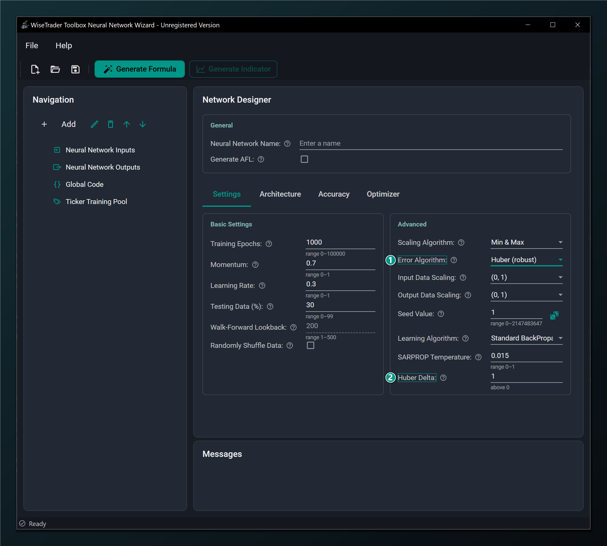
1. Error Algorithm set to Huber (robust) — makes regression robust to outliers.
2. Huber Delta — threshold where the Huber error switches from squared to linear. Only shown when Error Algorithm = Huber. Default 1.0.

Seed Value: making runs repeatable

A network starts from random weights, so two runs of the same design land in slightly different places. The Seed Value fixes that randomness, so the same seed gives the identical run every time. That's invaluable for fair comparisons — change one thing, re-train, and any difference in the result is down to your change, not a different roll of the dice. Roll the dice (or type a new number) to try a fresh starting point. Default 1.

Learning Algorithm: the training method

This chooses how the network learns from its errors. Standard BackPropagation is the safe, well-understood default. The RPROP / iRPROP variants adapt the step size for each weight automatically and often train faster and more reliably — a good second thing to try. SARPROP adds a touch of "annealing" (controlled randomness early on) to help escape poor starting spots. The modern Adam-family optimizers are powerful and are required for recurrent models.

Your choice here decides which extra knobs appear on the Optimizer tab: BackPropagation needs none, while the Adam-family optimizers reveal their own beta, epsilon and weight-decay fields and unlock the learning-rate schedules.

SARPROP Temperature

Only the SARPROP algorithm uses this. It's the strength of the early-training "annealing" — a controlled jitter that helps the network jump out of bad local solutions before settling down. Higher means more exploration early on. Typical values are 0.01–0.07; the default 0.015 is a good start (must be above 0 up to 1). Ignore this field unless you've selected SARPROP.